De novo design of functional nucleic acids of aptamers

Preparation of HT-SELEX data of TF-binding DNA for model training

The HT-SELEX datasets of ten TFs (Ar, Atf4, Dbp, Egr3, Foxg1, Klf12, Mlx, Nr2e1, Sox10 and Srebf1) used in this study were downloaded from the European Nucleotide Archive database (accession number: ERP001824)³⁵. The FASTQ files were further processed by removing the variable-length and redundant sequences, to obtain the cleaned sequences used for further continual pretraining of NA-LLM. The lengths and numbers of cleaned unique DNA sequences in each TF dataset are summarized in Supplementary Fig. 1.

Evaluating the binding specificity of TF-binding DNA sequences

The binding specificity score of TF to a DNA sequence is calculated using the 8mer_sum algorithm as described previously³⁶:

where S_total is the binding specificity score of the full-length DNA sequence, \({S}_{8\mathrm{mer}}^{i}\) is the protein-binding microarray fluorescence intensity of the ith 8-mer motif, which is extracted using a sliding window of length 8 and stride 1, and n represents the total number of 8-mer motifs in the full-length DNA sequence.

The relative binding specificity is normalized to a range from 0 to 100 using min–max normalization of binding specificity score:

where \({S}_{\min }\) and \({S}_{\max }\) represent the minimum and maximum binding specificity scores in the dataset, respectively. This scaling transforms the raw scores to the [0, 100] range.

InstructNA training and inference using DNABERT (3-mers)

Tokenization in DNABERT (3-mers)

In the domain of language modeling, tokens represent the fundamental semantic units that a model employs to interpret linguistic data. They can represent discrete units such as words or even more granular semantic elements such as individual characters. The act of tokenization involves transforming these linguistic units into unique integer identifiers, each corresponding to an entry within a reference lookup table. Subsequently, these integers are translated by embedding layers into vectorial representations, which the model then processes in a comprehensive, end-to-end manner. For the specific application within the InstructNA framework using DNABERT (3-mers), DNA sequences were tokenized using a trinucleotide (3-mers) resolution method. This approach results in a combinatorial diversity of 64 (4³) possible distinct 3-mers. Additionally, special utility tokens such as [CLS], [UNK], [SEP], [MASK] and [PAD] were integrated into the model for specific functional roles within the modeling process.

Training

The training process of InstructNA using DNABERT (3-mers) consists of two stages. In the first stage, we conducted continual pretraining on a pretrained DNABERT DNA-LLM using HT-SELEX data, with the training objective aligned with that of the original DNABERT pretraining (Supplementary Fig. 18). Specifically, 15% of the tokens were masked, and the model was trained to predict the masked tokens. To facilitate BO, a dimensionality reduction layer was incorporated during training, reducing the dimensionality of each token embedding to 8 (Supplementary Fig. 19). This process results in a domain-adapted FNA-LLM (encoder).

In the second stage, we froze the encoder and introduced a randomly initialized decoder composed of six-layer transformer blocks. We then performed a sequence reconstruction task, where HT-SELEX sequence data are fed into the model again. The encoder transformed these sequences into embeddings, which were subsequently passed to the decoder, enabling it to reconstruct the original sequence tokens. The objective of this training stage is to reconstruct the original input sequence from the embeddings. Specifically, the decoder outputs a vector of logits for the ith position token based on the corresponding embedding e_i, and a softmax layer is applied to obtain the probability distribution over the vocabulary. The loss function for this stage is

where P(x_i|e_i) represents the probability assigned to the ground-truth token x_i given the embedding e_i after the softmax transformation.

Inference

Using embeddings derived from clustering centers or BO, the decoder processes these embeddings to produce an initial generated sequence. Next, the 15% of tokens with the lowest probabilities in this sequence were replaced with a special token, [MASK], and the modified sequence was fed back into the encoder to predict and refine the masked-out portions. This iterative refinement process is repeated several times, progressively enhancing the accuracy of the generated sequence.

HC-HEBO in InstructNA

The HC-HEBO algorithm combines HC with HEBO to efficiently optimize FNAs.

1. (1)

   Initial solution construction. Sequences from diverse sources are evaluated and their embeddings are denoted as E₀ = {e₀, e₁, e₂,…,e_n}. E₀ is divided into n groups and each e_i ∈ E₀ (0 ≤ i ≤ n) represents the initial solution for the group respectively.

2. (2)

   Search space definition. For the n groups, define the initial search space as a neighborhood centered around E₀, with a search radius R₀ (default ΔR₀ = 5). The sensitivity experiment of the search radius and minimum threshold is shown in Supplementary Fig. 20. The n initial search space S₀ = {s₀, s₁, s₂, …, s_n} is defined as

   $${E}_{0}\,({\rm{initial}}\,{\rm{solution}})$$

   (4)

   $${S}_{0}=\{\mathbf{e}|\parallel \mathbf{e}-{E}_{0}\parallel \le \Delta {R}_{0}\}\,({\rm{initial}}\,{\rm{search}}\,{\rm{space}}).$$

   (5)

3. (3)

   Searching and generation. Use HEBO to search next embeddings in the search space with the hyperparameters in HEBO kept as default. InstructNA generates and evaluates a total of n new sequences, with one new sequence generated per group.

4. (4)

   Greedy refinement. At each iteration, the solution (embedding) with the best evaluated performance within its group is chosen as the candidate solution for the next optimization. The ith group solution obtained at the tth iteration is E_i,t:

   $${\mathbf{E}}_{i,t}=\text{arg}\mathop{\max }\limits_{\textbf{e}\in {G}_{t,i}}f(\textbf{e})$$

   (6)

   where G_t,i represents the ith group of evaluated solutions at iteration t and f(e) represents the evaluated performance.

5. (5)

   Shrinking search radius. After each iteration, the search radius is reduced by half, but once it reaches a minimum threshold ΔR_min (default ΔR_min = 1.25), the search radius will no longer shrink and remains constant:

   $${S}_{t+1}=\left\{\textbf{e}|\Vert \textbf{e}-{E}_{t}\Vert \le \frac{\Delta {R}_{t}}{2}\right\},\,\mathrm{if}\,\Delta {R}_{t} > \Delta {R}_{\min }$$

   (7)

   $${S}_{t+1}=\{\mathbf{e}|\Vert \mathbf{e}-{E}_{t}\Vert \le \Delta {R}_{\min }\},\,\mathrm{if}\,\Delta {R}_{t}\le \Delta {R}_{\min }.$$

   (8)

6. (6)

   Obtain the tth iteration best solution E_t, search space S_t. Repeat steps 3–5 for iteration.

Assessing correlation between embeddings and sequences

We randomly sampled 1,000 unique sequences from the HT-SELEX dataset. From these sequences, we generated all possible pairs (\({C}_{1,000}^{2}\)), resulting in a total of 499,500 sequence pairs. We explored the relationship between sequences and embeddings by analyzing the cosine similarity and pairwise alignment similarity of these sequence pairs.

Cosine similarity calculation

For InstructNA and DNABERT, we calculated the cosine similarity of token embeddings at corresponding positions for each pair of sequences, and then averaged the cosine similarities across all tokens to obtain the final cosine similarity score representing the full embedding similarity of the sequence pair.

where S₁ and S₂ represent the sequences in the sequence pair, \({\mathbf{e}}_{i}^{1}\) and \({\mathbf{e}}_{i}^{2}\) represent the embedding of the ith token in S₁ and S₂, and · denotes the vector inner product.

For RaptGen, we compute the cosine similarity between the 2D embeddings of sequence pairs directly.

Sequence similarity

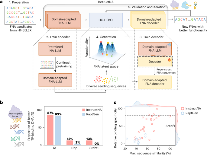
Sequence similarity is calculated using the EMBOSS Needle tool⁴⁸ that creates an optimal global alignment of two sequences using the Needleman–Wunsch algorithm with default parameters: matrix = DNA full, gap open penalty = 10, gap extended penalty = 0.5, end gap open penalty = 10 and end gap extend penalty = 0.5. For the DNA sequences binding to TFs, the sequence similarity is calculated on the 14-nucleotide or 20-nucleotide random DNA (Supplementary Fig. 1). For the DNA aptamers binding to LOX1 or CXCL5, the sequence similarity is calculated on the 36-nucleotide random DNA (Supplementary Table 2).

Binary classification of binding specificity

For the cleaned unique sequences in each TF dataset as shown in Supplementary Fig. 1, we cluster them using cd-hit⁴⁹ at an 80% sequence similarity cutoff^18,50, collect representative sequences from each cluster and randomly split the collected sequences into training (40%), validation (10%) and test (50%) sets. The numbers of sequences in training, validation and test sets are summarized in Supplementary Table 1. On the basis of the median binding specificity score in the training and validation sets, we label each sequence as 0 (low binding specificity) or 1 (high binding specificity) and train the model.

In the classification pipeline, encoders pretrained by InstructNA and RaptGen remain frozen, with a trainable linear layer appended for binary classification. Model performance is assessed on the test set using the following metrics:

where TP, TN, FP and FN represent true positive, true negative, false positive and false negative respectively in the confusion matrix.

KDE perturbation generation experiment

A perturbation generation experiment was performed separately on the ten HT-SELEX datasets of TF-binding DNA sequences. The embeddings of all DNA sequences from each HT-SELEX dataset were obtained using the InstructNA and RaptGen encoders. These embeddings were then used to train a KDE³⁷ model to learn the probability density distribution of the embeddings. Two thousand new embeddings were sampled from the trained KDE model based on the learned probability density function. These new embeddings were input into the decoder for inference. Finally, InstructNA and RaptGen generated 2,000 sequences for each HT-SELEX dataset, respectively. For the real sequences, we performed stratified sampling to select 2,000 sequences on the basis of sequence frequency from each HT-SELEX dataset. Then, k-mer frequency and G/C content of these sequences were calculated. The k-mer counts were obtained using sliding windows of lengths 3–6 with a stride of 1 for each sequence, and frequency was calculated on the basis of the k-mer counts. The G/C content was determined by calculating the proportion of G and C nucleotides in each sequence.

Pipeline of InstructNA to generate new DNA sequences for TF binding

To generate new DNA sequences that have high binding specificity to a TF, we trained InstructNA as stated above. During the generation and optimization by HC-HEBO, 30 starting seeds were collected from three sources, including ten top-frequency sequences in the original HT-SELEX data (S1), ten sequences decoded from each of the ten cluster centers of the entire HT-SELEX embeddings clustered by the Gaussian mixture model (GMM)⁵¹ (S2) and ten sequences with similar embeddings (calculated by the minimum Euclidean distance) to the DNAs with the highest binding specificity from S1 and S2 (S3). Notably, the number of seeding sequences can vary. The 30 candidates were then clustered into ten clusters using GMM, and the sequence of the highest binding specificity score in each group was chosen to constitute the initial ten seeding sequences for HC-HEBO.

HT-SELEX for screening protein-binding DNA aptamers

The ssDNA library and primers shown in Supplementary Table 2 were purchased from Sangon Biotech. The ssDNA library was denatured at 95 °C for 10 min, 4 °C for 6 min and 25 °C for 2 min. COOH-modified magnetic beads (400 μl; Zecen Biotech) were washed with 1 ml of 10-mM NaOH once and 1 ml of double-distilled water twice, and activated in 800 μl of 0.4-M 1-(3-dimethylaminopropyl)-3-ethylcarbodiimide (EDC) and 0.1-M N-hydroxysuccinimide (NHS) (1:1, v/v) for 15 min. Then, ~80 μg of protein (PTM Bio) diluted in sodium acetate was added to the magnetic beads and incubated for 2 h. Supernatant was discarded and the beads were washed three times with 1 ml of Dulbecco’s phosphate-buffered saline (DPBS). Then, the beads were blocked in 1 ml of 10 mM ethanolamine (pH 8.0), incubated for 15 min, washed three times with 800 μl of 1× washing buffer and then resuspended in 400 μl of antibody diluent buffer.

Each round of counter-selection and positive selection was conducted using the conventional magnetic bead-based HT-SELEX method. The His–magnetic beads were washed with 1× DPBS, and then incubated with the ssDNA library for 1 h. The mixture was washed with 1× washing buffer, and then the His–magnetic beads were discarded, leaving the remaining DNA pool for positive selection. DNAs bound to the target protein were eluted by boiling the protein–magnetic beads in 100 μl of double-distilled water at 95 °C for 10 min, amplified with PCR using rTaq DNA polymerase (Takara) and used for the next round of selection. For PCR amplification, we used MIX configuration with the forward primer and biotin-modified reverse primer, and the ssDNA eluted from the positive selection as the template. Double-stranded DNA (1 ml) obtained from PCR was incubated with 80 μl of streptavidin-modified magnetic beads (Smart-Lifesciences Biotech) in 1-M NaCl for 30 min, washed with 1× washing buffer three times and treated with 100 μl of 40-mM NaOH. The biotin-modified strands left on streptavidin-modified magnetic beads were removed by magnetic suction, neutralized with 4 μl of 1-M HCl and combined with an equal volume of 2× DPBS buffer. For high-throughput sequencing, each round of the ssDNA library was amplified using the forward and reverse primers, followed by the use of a standard library construction kit (E7335S NEB). Polyclonal amplicons were purified using VAHTS DNA Clean Beads (Vazyme) following the manufacturer’s protocol, quantified with QUBIT (Invitrogen). The sequencing was performed using the GeneMind sequencer. The high-throughput sequencing data from the last round of SELEX were used for InstructNA.

Pipeline of InstructNA to generate DNA aptamers

The last round of aptamer HT-SELEX data was used to train InstructNA as stated above. The 30 seeding sequence candidates from S1, S2 and S3 were engineered in the same way as stated above for those of TF-binding DNAs. The 30 candidate sequences were clustered into ten clusters using GMM, and the sequence with the smallest K_D measured by SPR to the target protein was chosen to constitute the initial seeding sequences for HC-HEBO optimization.

SPR experiments

The DNA oligonucleotides used for SPR experiments shown in Supplementary Tables 3–6 were purchased from Sangon Biotech. The SPR experiments were performed on a Biacore 8K instrument (GE Healthcare). The sensor chip (CM5, Cytiva) was activated by injecting a 50:50 (v/v) mixture of NHS (0.1 M) and EDC (0.4 M) for 5 min. The protein (50 µg ml⁻¹) was diluted in sodium acetate and injected into flow cell 2 at a flow rate of 10 µl min⁻¹ for 5 min. Next, the His protein (5 µg ml⁻¹) diluted in sodium acetate was injected into flow cell 1 as a control channel. Finally, the sensor chip was blocked using ethanolamine-HCl (1 M, pH 8.5) for 2 min. The DNA aptamers were diluted to different concentrations using 1× PBS containing 5-mM magnesium chloride. Aptamers at various concentrations in running buffer (DPBS supplemented with 5-mM MgCl₂) were injected into the analyte channel at a flow rate of 30 μl min⁻¹, a contact time of 120 s and a dissociation time of 120 s. After each analysis cycle, the analyte channels were regenerated via a 30-s injection of 1.5-M NaCl. The K_D was obtained by fitting the sensorgram with a 1:1 binding model using Biacore evaluation software (GE Healthcare).

Docking and unrestrained MD simulations

The AlphaFold3 webserver (https://alphafoldserver.com/) was utilized to predict the 3D structures of DNA aptamers T1^L, G1^L (nucleotides 1–76) and LOX1 (amino acids 61–237), which are consistent with the sequence lengths used in SPR experiments. Initially, we attempted to predict the complex structure directly from the input protein and DNA sequences, but the resulting structures were visibly not bound together. Therefore, on the basis of the monomer structures of the protein and DNAs, the LOX1–T1^L and LOX1–G1^L complexes were obtained via the molecular docking using HDOCKlite v.1.1, based on a hybrid algorithm of template-based modeling and ab initio free docking. The LOX1 protein was set as the receptor, and the DNA aptamer was treated as the ligand. Blind docking was performed, and the top docking pose based on the docking score was selected as the initial structure for MD simulations.

The complex structure was subjected to unrestrained MD simulations on the Amber22 package. The complex was modeled using the tleap module in Amber22. The Amber ff19SB force field was used for the protein and the OL15 force field was employed for DNA. After adding Na⁺ to neutralize the phosphate backbone charges, the system was then solvated with TIP3P water in a 12-Å cuboid box. Initial minimizations were carried out with 2,000 steps of steepest descent followed by 3,000 steps of conjugated gradient, during which the DNA positions were fixed. The particle mesh Ewald algorithm was employed to efficiently treat the long-range electrostatic interaction. Then the system was heated to 300 K under constant volume in 50 ps, followed by a 50-ps constant-pressure relaxation using the Langevin thermostat at 300 K. All covalent bonds involving hydrogen atoms were constrained using the SHAKE algorithm. The cutoff was set to 12.0 Å for the electrostatic and van der Waals interactions. The final production was performed at 300 K without restraints on DNA for 100 ns. Ten independent runs of MD simulations were performed for each complex.

Statistics and reproducibility

No statistical method was used to predetermine sample size. No data were excluded from the analyses. Training, validation and test sets for training models of binary classification were generated via random splits of the full datasets. No randomization was applied in the comparative experiments. Blinding was not relevant to this study.

Reporting summary

Further information on research design is available in the Nature Portfolio Reporting Summary linked to this article.