Bayesian statistics you’ve likely encountered MCMC. While the rest of the world is fixated on the latest LLM hype, Markov Chain Monte Carlo remains the quiet workhorse of high-end quantitative finance and risk management. It is the tool of choice when “guessing” isn’t enough and you need to rigorously map out uncertainty.
Despite the intimidating acronym, Markov Chain Monte Carlo is a combination of two straightforward concepts:
- A Markov Chain is a stochastic process where the next state of the system depends entirely on its current state and not on the sequences of events that preceded it. This property is usually referred to asmemorylessness.
- A Monte Carlo method simply refers to any algorithm that relies on repeated random sampling to obtain numerical results.
In this series, we will present the core algorithms used in MCMC frameworks. We primarily focus on those used for Bayesian methods.
We begin with Metropolis-Hastings: the foundational algorithm that enabled the field’s earliest breakthroughs. But before diving into the mechanics, let’s discuss the problem MCMC methods help solve.
The Problem
Suppose we want to be able to sample variables from a probability distribution which we know the density formula for. In this example we use the standard normal distribution. Let’s call a function that can sample from it rnorm.
For rnorm to be considered helpful, it must generate values \(x\) over the long run that match the probabilities of our target distribution. In other words, if we were to let rnorm run \(100,000\) times and if we were to collect these values and plot them by the frequency they appeared (a histogram), the shape would resemble the standard normal distribution.
How can we achieve this?
We start with the formula for the unnormalised density of the normal distribution:
\[p(x) = e^{-\frac{x^2}{2}}\]
This function returns a density for a given \(x\) instead of a probability. To get a probability, we need to normalise our density function by a constant, so that the total area under the curve integrates (sums) to \(1\).
To find this constant we need to integrate the density function across all possible values of \(x\).
\[C = \int^\infty_{-\infty}e^{-\frac{x^2}{2}}\,dx\]
There is no closed-form solution to the indefinite integral of \(e^{-x^2}\). However, mathematicians solved the definite integral (from \(-\infty\) to \(\infty\)) by moving to polar coordinates (because apparently, turning a \(1D\) problem to a \(2D\) one makes it easier to solve) , and realising the total area is \(\sqrt{2\pi}\).
Therefore, to make the area under the curve sum to \(1\), the constant must be the inverse:
\[C = \frac{1}{\sqrt{2\pi}}\]
This is where the well-known normalisation constant \(C\) for the normal distribution comes from.
OK great, we have the mathematician-given constant that makes our distribution a valid probability distribution. But we still need to be able to sample from it.
Since our scale is continuous and infinite the probability of getting exactly a specific number (e.g. \(x = 1.2345…\) to infinite precision) is actually zero. This is because a single point has no width, and therefore contains no ‘area’ under the curve.
Instead, we must speak in terms of ranges i.e. what is the probability of getting a value \(x\) that falls between \(a\) and \(b\) (\(a < x < b\)), where \(a\) and \(b\) are fixed values?
In other words, we need to find the area under the curve between \(a\) and \(b\). And as you’ve correctly guessed, to calculate this area we typically need to integrate our normalised density formula – the resulting integrated function is known as the Cumulative Distribution Function (\(CDF\)).
Since we cannot solve the integral, we cannot derive the \(CDF\) and so we’re stuck again. The clever mathematicians solved this too and have been able to use trigonometry (specifically the Box-Muller transform) to convert uniform random variables to normal random variables.
But here is the catch: In the real world of Bayesian statistics and machine learning, we deal with complex multi-dimensional distributions where:
- We cannot solve the integral analytically.
- Therefore we cannot find the normalisation constant \(C\)
- Finally, without the integral, we cannot calculate the CDF, so standard sampling fails.
We are stuck with an unnormalised formula and no way to calculate the total area. This is where MCMC comes in. MCMC methods allow us to sample from these distributions without ever needing to solve that impossible integral.
Introduction
A Markov process is uniquely defined by its transition probabilities \(P(x\rightarrow x’)\).
For example in a system with \(4\) states:
\[P(x\rightarrow x’) = \begin{bmatrix} 0.5 & 0.3 & 0.05 & 0.15 \\ 0.2 & 0.4 & 0.1 & 0.3 \\ 0.4 & 0.4 & 0 & 0.2 \\ 0.1 & 0.8 & 0.05 & 0.05 \end{bmatrix}\]
The probability of going from any state \(x\) to \(x’\) is given by entry \(i \rightarrow j\) in the matrix.
Look at the third row, for instance: \([0.4,0.4,0,0.2]\).
It tells us that if the system is currently in State \(3\), it has a \(40\%\) chance of moving to State \(1\), a \(40\%\) chance of moving to State \(2\), a \(0\%\) chance of staying in State \(3\), and a \(20\%\) chance of moving to State \(4\).
The matrix has mapped every possible path with its corresponding probabilities. Notice that each row \(i\) sums to \(1\) so that our transition matrix represents valid probabilities.
A Markov process also requires an initial state distribution \(\pi_0\) (do we start in state \(1\) with \(100\%\) probability or any of the \(4\) states with \(25\%\) probability each?).
For example, this could look like:
\[\pi_0 = \begin{bmatrix} 0.4 & 0.15 & 0.25 & 0.2 \end{bmatrix}\]
This simply means the probability of starting from state \(1\) is \(0.4\), state \(2\) is \(0.15\) and so on.
To find the probability distribution of where the system will be after the first step \(t_0 + 1\), we multiply the initial distribution with the transition probabilities:
\[ \pi_1 = \pi_0P\]
The matrix multiplication effectively gives us the probability of all the routes we can take to get to a state \(j\) by summing up all the individual probabilities of reaching \(j\) from different starting states \(i\).
Why this works
By using matrix multiplication we are exploring every possible path to a destination and summing their likelihood.
Notice that the operation also beautifully preserves the requirement that the sum of the probabilities of being in a state will always equal \(1\).
Stationary Distribution
A properly constructed Markov process reaches a state of equilibrium as the number of steps \(t\) approaches infinity:
\[\pi^* P = \pi^*\]
Such a state is known as global balance.
\(\pi^*\) is known as the stationary distribution and represents a time at which the probability distribution after a transition (\(\pi^*P\)) is identical to the probability distribution before the transition (\(\pi^*\)).
The existence of such a state happens to be the foundation of every MCMC method.
When sampling a target distribution using a stochastic process, we aren’t asking “Where to next?” but rather “Where do we end up eventually?”. To answer that, we need to introduce long term predictability into the system.
This guarantees that there exists a theoretical state \(t\) at which the probabilities “settle” down instead of moving in random for all eternity. The point at which they “settle” down is the point at which we hope we can start sampling from our target distribution.
Thus, to be able to effectively estimate a probability distribution using a Markov process we need to ensure that:
- there exists a stationary distribution.
- this stationary distribution is unique, otherwise we could have multiple states of equilibrium in a space far away from our target distribution.
The mathematical constraints imposed by the algorithm make a Markov process satisfy these conditions, which is central to all MCMC methods. How this is achieved may vary.
Uniqueness
In general, to guarantee the uniqueness of the stationary distribution, we need to satisfy three conditions. Expand the section below to see them:
The Holy Trinity
- Irreducible: A system is irreducible if at any state \(x\) there is a non-zero probability of any point \(x’\) in the sample space being visited. Simply put, you can get from any state A to any state B, eventually.
- Aperiodic: The system must not return to a particular state in fixed intervals. A sufficient condition for aperiodicity is that there exists at least one state where the probability of staying is non-zero.
- Positive Recurrent: A state \(x\) is positive recurrent if starting from that state the system is guaranteed to return to it and the average number of steps it takes to return to is finite. This is assured by us modelling a target that has a finite integral and is a proper probability distribution (the area under the curve must sum to \(1\)).
Any system that meets these conditions is known as an ergodic system. The tables at the end of the article show how the MH algorithm deals with ensuring ergodicity and therefore uniqueness.
Metropolis-Hastings
The approach the MH algorithm takes is to begin with the definition of detailed balance – a sufficient but not not necessary condition for global balance. Quite simply, if our algorithm satisfies detailed balance, we will guarantee that our simulation has a stationary distribution.
Derivation
The definition of detailed balance is:
\[\pi(x) P(x’|x) = \pi(x’) P(x|x’) ,\]
this means that the probability flow of going from \(x\) to \(x’\) is the same as the probability flow going from \(x’\) to \(x\).
The idea is to find the stationary distribution by iteratively building the transition matrix, \(P(x’,x)\) by setting \(\pi\) to be the target distribution \(P(x)\) we want to sample from.
To implement this, we decompose the transition probability \(P(x’|x)\) into two separate steps:
- Proposal (\(g\)): The probability of proposing a move to \(x’\) given we are at \(x\).
- Acceptance (\(A\)): The acceptance function gives us the probability of accepting the proposal.
Thus,
\[P(x’|x) = g(x’|x) a(x’,x)\]
The Hastings Correction
Substituting these values back into the equation above gives us:
\[\frac{\pi(x)}{\pi(x’)} = \frac{g(x|x’) a(x,x’)}{g(x’|x) a(x’,x)}\]
and finally rearranging we get an expression for our acceptance as a ratio:
\[\frac{a(x’,x)}{a(x,x’)} = \frac{g(x|x’)\pi(x’)}{g(x’|x)\pi(x)}\]
This ratio represents how much more likely we are to accept a move to \(x’\) compared to a move back to \(x\).
The \(\frac{g(x|x’)\pi(x’)}{g(x’|x)\pi(x)}\) term is known as the Hastings correction.
Important Note
Because we often choose a symmetric distribution for the proposal, the probability of jumping from \(x \rightarrow x’\) is the same as jumping from \(x’ \rightarrow x\). Therefore, the proposal terms cancel each other out leaving only the ratio of the target densities.
This special case where the proposal is symmetric and the \(g\) terms vanish is historically known as the Metropolis Algorithm (1953). The more general version that allows for asymmetric proposals (requiring the \(g\) ratio – known as the Hastings correction) is the Metropolis-Hastings Algorithm (1970).
The Breakthrough
Recall the original problem: we cannot calculate \(\pi(x)\) because we don’t know the normalisation constant \(C\) (the integral).
However, look closely at the ratio \(\frac{\pi(x’)}{\pi(x)}\). If we expand \(\pi(x)\) into its unnormalised density \(f(x)\) and the constant \(C\):
\[\frac{\pi(x’)}{\pi(x)} = \frac{{f(x’)} / C}{f(x) / C} = \frac{f(x’)}{f(x)}\]
The constant \(C\) cancels out!
This is the breakthrough. We can now sample from a complex distribution using only the unnormalised density (which we know) and the proposal distribution (which we choose).
All that’s left to do is to find an acceptance function \(A\) that will satisfy detailed balance:
\[\frac{a(x’,x)}{a(x,x’)} = R ,\]
where \(R\) represents \(\frac{g(x|x’)\pi(x’)}{g(x’|x)\pi(x)}\).
The Metropolis Acceptance
The acceptance function the algorithm uses is:
\[a(x’,x) = \min(1,R)\]
This ensures that the acceptance probability is always between \(0\) and \(1\).
To see why this choice satisfies detailed balance, we must verify that the equation holds for the reverse move as well. We need to verify that:
\[\frac{a(x’,x)}{a(x,x’)} = R,\]
in two cases:
Case I: The move is advantageous (\(R \ge 1\))
Since \(R \ge 1\), the inverse \(\frac{1}{R} \le 1\):
- our forward acceptance is \(a(x’,x) = \min(1,R) = 1\)
- our reverse acceptance is \(a(x,x’) = \min(1,\frac{1}{R}) = \frac{1}{R}\)
\[\frac{1}{a(x,x’)} = R\]
\[\frac{1}{\frac{1}{R}} = R\]
Case II: The move is not advantageous (\(R < 1\))
Since \(R < 1\), the inverse \(\frac{1}{R} > 1\):
- our forward acceptance is \(a(x’,x) = \min(1,R) = R\)
- our reverse acceptance is \(a(x,x’) = \min(1,\frac{1}{R}) = 1\)
Thus:
\[\frac{R}{a(x,x’)} = R\]
\[\frac{R}{1} = R,\]
and the equality is satisfied in both cases.
Implementation
Lets implement the MH algorithm in python on two example target distributions.
I. Estimating a Gaussian Distribution
When we plot the samples on a chart against a true normal distribution this is what we get:

Now you might be thinking why we bothered running a MCMC method for something we can do using np.random.normal(n_iterations). That is a very valid point! In fact, for a 1-dimensional Gaussian, the inverse-transform solution (using trignometry) is much more efficient and is what numpy actually uses.
But at least we know that our code works! Now, let’s try something more interesting.
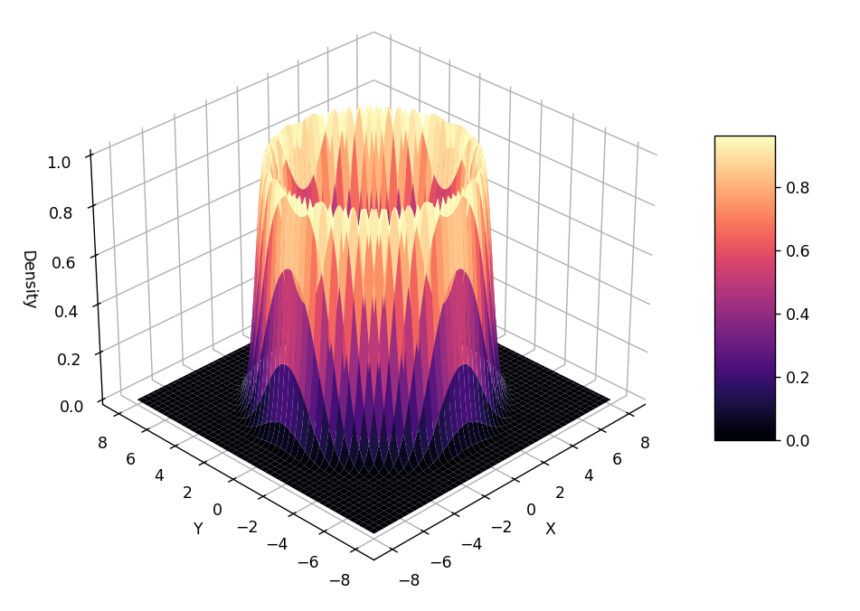
II. Estimating the ‘Volcano’ Distribution
Let’s try to sample from a much less ‘standard’ distribution that is constructed in 2-dimensions, with the third dimension representing the distribution’s density.
Since the sampling is happening in \(2D\) space (the algorithm only knows its x-y location not the ‘slope’ of the volcano) – we get a pretty ring around the mouth of the volcano.

Summary of Mathematical Conditions for MCMC
Now that we’ve seen the basic implementation here’s a quick summary of the mathematical conditions an MCMC method requires to actually work:
| Condition | Mechanism |
|---|---|
| Stationary Distribution (That there exists a set of probabilities that, once reached, will not change.) |
Detailed Balance The algorithm is designed to satisfy the detailed balance equation. |
| Convergence (Guaranteeing that the chain eventually converges to the stationary distribution.) |
Ergodicity The system must satisfy the conditions in table 2 be ergodic. |
| Uniqueness of Stationary Distribution (That there exists only one solution to the detailed balance equation) |
Ergodicity Guaranteed if the system is ergodic. |
And here’s how the MH algorithm satisfies the requirements for ergodicity:
| Condition | Mechanism |
|---|---|
| 1. Irreducible (Ability to reach any state from any other state.) |
Proposal Function Often satisfied by using a proposal (like a Gaussian) that has non-zero probability everywhere. Note: If jumps to some regions are not possible, this condition fails. |
| 2. Aperiodic (The system does not get trapped in a loop.) |
Rejection Step The “coin flip” allows us to reject a move and stay in the same state, breaking any periodicity that may have occurred. |
| 3. Positive Recurrent (The expected return time to any state is finite.) |
Proper Probability Distribution Guaranteed by the fact that we model the target as a proper distribution (i.e., it integrates/sums to \(1\)). |
Conclusion
In this article we have seen how MCMC helps solve the two main challenges of sampling from a distribution given only its unnormalised density (likelihood) function:
- The normalisation problem: For a distribution to be a valid probability distribution the area under the curve must sum to \(1\). To do this we need to calculate the total area under the curve and then divide our unnormalised values by that constant. Calculating the area involves integrating a complex function and in the case of the normal distribution for example no closed-form solution exists.
- The inversion problem: To generate a sample we need to pick a random probability and ask what \(x\) value corresponds to this area? To do this we not only have to solve the integral but also invert it. And since we can’t write down the integral it is impossible to solve its inverse.
MCMC methods, starting with Metropolis-Hastings, allow us to bypass these impossible math problems by using clever random walks and acceptance ratios.
For a more robust implementation of the Metropolis-Hastings algorithm and an example of sampling using an asymmetric proposal (utilising the Hastings correction) check out the go code here.
What’s Next?
We’ve successfully sampled from a complex \(2D\) distribution without ever calculating an integral. However, if you look at the Metropolis-Hastings code, you’ll notice our proposal step is essentially a blind, random guess (np.random.normal).
In low dimensions, guessing works. But in the high-dimensional spaces of modern Bayesian methods, guessing randomly is like trying to get a better rate from a usurer – almost every proposal you make will be rejected.
In Part II, we will introduce Hamiltonian Monte Carlo (HMC), an algorithm that allows us to efficiently explore high-dimensional space using the geometry of the distribution to guide our steps.