Summarize this content to 100 words:
Author(s): Mohamed Bedhiafi
Originally published on Towards AI.
Moving beyond brittle fallback rules toward a mathematically principled, learnable healing system
Your test suite passes on Friday. On Monday, a developer renames a CSS class, shuffles a form layout — and suddenly 40 automated tests are failing. Not because the application broke. Because your XPaths did.
This is the quiet crisis of test automation at scale. And the industry’s standard answer — self-healing — is smarter than nothing, but not nearly smart enough.
Why Heuristic Healing Fails
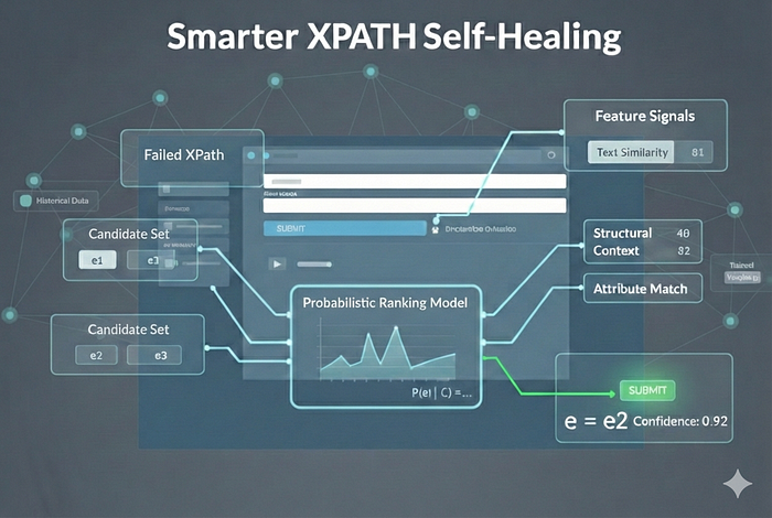
Most self-healing tools work like this: when an XPath fails, walk down a ranked list of fallback strategies.
1. Try by ID2. Try by name attribute 3. Try by visible text4. Try by CSS class…
It sounds reasonable. In practice, it’s a house of cards — and the failure modes are structural, not incidental.
Static priority is context-blind. An ID match sounds like a slam dunk, until your frontend auto-generates IDs like input_3847291. Class names sound stable until a design system refactor renames btn-primary to button–cta. No heuristic knows which signals are reliable in your specific application.
Strategies are evaluated in isolation. A good healing decision fuses multiple signals: the text looks right and the parent tag matches and the depth is similar. Heuristic ladders evaluate signals one at a time and stop at the first hit — they can’t combine evidence.
There is no learning. Every healing event is stateless. The system makes the same mistakes repeatedly, never improving from a growing history of successes and failures.
Confidence is binary. Either a fallback finds something or it doesn’t. There’s no probability score, no uncertainty estimate, no threshold to tune.
The fundamental problem: heuristic healing is a lookup table pretending to be intelligence.
Reframing the Problem Formally
Let’s state the problem precisely, because precision is where the solution lives.
At time t−1, a test correctly targets element e* in the DOM D(t−1). At time t, the DOM has evolved into D(t), the original XPath fails, and we need to identify the element that most likely corresponds to e*.
Formally, we want:
ê = argmax P(e = e* | D_t, φ*)e ∈ D_t
Where φ* is a feature representation extracted from the original element — its attributes, visible text, structural position, surrounding context. This is not a lookup problem. It is a ranking problem over a probability distribution on the current DOM.
Step 1 — Candidate Set Construction
Before any scoring, we prune the search space. Evaluating every element in a modern DOM (often 1,000+ nodes) is wasteful and injects noise. We define a candidate filter:
C = { e ∈ D_t | candidate_filter(e, φ*) = 1 }
The filter is intentionally cheap and permissive — same tag, matching type or role, any text overlap. Its job is elimination, not selection. The probabilistic model handles selection.
def build_candidate_set(dom, target):return [el for el in dom.find_all()if el.name == target.tag and (any(el.get(a) == target.attrs.get(a) for a in [‘type’, ‘role’, ‘name’] if target.attrs.get(a))or any(w in el.get_text() for w in target.visible_text.split()[:3]))]
Step 2 — Feature Representation
The heart of the system is a function ψ(e, φ*) that maps each candidate element and the original element’s snapshot into a numeric feature vector:
x_e = ψ(e, φ*) ∈ ℝᵈ
We decompose this into four groups of signals.
A — Attribute Similarity
We compare element attributes between the candidate and the original target. Key features:
ID exact match:
x_id = 𝟙(id_e = id*)
Class Jaccard similarity — measures set overlap between class lists:
x_class = |C_e ∩ C*| / |C_e ∪ C*|
Fuzzy attribute matching for name, placeholder, and aria-label using sequence similarity. Together these form the attribute sub-vector:
x_attr = [x_id, x_class, x_name, x_type, x_placeholder, …]
B — Text Similarity
Visible text is often the most stable signal — labels survive refactors because users see them. We use two measures:
Exact match:
x_text_exact = 𝟙(T_e = T*)
Semantic cosine similarity via sentence embeddings — captures meaning even when wording shifts slightly:
x_text_cos = v(T_e) · v(T*) / (‖v(T_e)‖ ‖v(T*)‖)
C — Structural Similarity
Where an element lives in the DOM tree is often more stable than its attributes. We define the DOM as a graph G = (V, E) and extract:
Depth difference — normalized distance from root:
x_depth = |depth(e) – depth(e*)|
Parent tag match:
x_parent = 𝟙(tag(parent(e)) = tag(parent(e*)))
Tree edit distance between local subtrees, capturing structural neighborhood:
x_tree = TreeEditDistance(subtree(e), subtree(e*))
D — Context Similarity
The label next to a button, the heading above a form — nearby text is often the most durable anchor of all. We define the k-neighborhood N_k(e) as siblings and parent text, then compute:
x_context = cos(v(context_e), v(context*))
The full feature vector is the concatenation of all four groups:
x_e = [ x_attr | x_text | x_struct | x_context ]
Step 3 — The Probabilistic Ranking Model
Here is where the approach diverges fundamentally from heuristics.
Rather than score candidates independently, we rank them against each other using a softmax ranking model (also known as the Plackett-Luce model). For a healing event with candidate set C = {e₁, e₂, …, eₙ}, the probability that eᵢ is the correct match is:
P(eᵢ | C) = exp(wᵀ x_eᵢ) / Σⱼ exp(wᵀ x_eⱼ)
This formulation has a crucial property: scores compete within the candidate set. Probabilities always sum to 1 and reflect relative confidence — not just absolute similarity to a fixed threshold. The model knows that choosing e₃ means not choosing e₁ and e₂.
The decision rule is then clean and interpretable:
ê = argmax wᵀ x_e (selection)e ∈ C
Confidence = P(ê | C) (uncertainty quantification)
And we heal conditionally:
Heal only if Confidence > τ
The threshold τ becomes a tuneable dial between precision and recall — something heuristic systems simply cannot offer.
Step 4 — Training the Model
We learn the weight vector w from historical healing events. Each event contributes one correct element (label = 1) and several incorrect candidates (label = 0).
The training objective is cross-entropy loss over the correct element within each candidate set:
L = -Σᵢ log P(e_correct | Cᵢ)
With L2 regularization to prevent overfitting:
L_total = -Σᵢ log P(e_correct | Cᵢ) + λ ‖w‖²
This is implemented straightforwardly as logistic regression over the feature matrix:
from sklearn.linear_model import LogisticRegressionfrom sklearn.preprocessing import StandardScaler
scaler = StandardScaler()X_scaled = scaler.fit_transform(X) # X: (n_candidates, d) feature matrixmodel = LogisticRegression(C=1.0/λ, class_weight=’balanced’)model.fit(X_scaled, y) # y: binary labels
After training, inspect model.coef_ to see what the model actually learned. If x_class_jaccard has high weight, your app uses stable class names. If x_context_cosine dominates, surrounding labels are your most reliable anchors. The learned weights are a diagnostic — they reveal real facts about your frontend’s stability structure.
Step 5 — Bayesian Prior Integration
One final enrichment. Not all element types are equally stable across changes. Buttons survive refactors better than auto-generated list items. Form inputs outlast decorative divs.
We encode this as a prior over element types — the historical healing success rate — and fold it into the score via log-odds adjustment:
score(e) = wᵀ x_e + log P(e)
Where:
P(e) = (successes_for_tag + α) / (total_for_tag + 2α) [Laplace smoothed]
This is Bayesian inference in its cleanest form: the likelihood from our feature model, multiplied by the prior from historical experience. The system learns not just how to match elements, but which kinds of elements are worth trusting.
The Full Pipeline
Putting it all together, the healing system becomes a five-step pipeline:
Given: failed XPath, previous DOM snapshot, current DOM1. φ* ← extract_snapshot(failed_xpath, previous_dom)2. C ← candidate_filter(current_dom, φ*)3. For each e ∈ C: x_e = ψ(e, φ*)4. s_e = wᵀ x_e + log P(e)5. P(e|C) = exp(s_e) / Σⱼ exp(sⱼ)ê = argmax s_eHeal if P(ê|C) > τ, else escalate
The entire system is now:
Supervised — it learns from your application’s actual healing history
Probabilistic — every decision comes with a calibrated confidence score
Interpretable — feature weights reveal which signals matter in your codebase
Adaptive — retrain on new events and the model evolves with your frontend
What This Unlocks in Practice
Confidence thresholds become meaningful. Set τ = 0.80 in production for high-precision healing. Drop to τ = 0.50 in CI for higher coverage. The tradeoff is explicit and controllable.
Human-in-the-loop escalation. When confidence is low, surface the top 3 candidates with their probabilities to a reviewer. Uncertainty triggers the right action rather than a silent wrong one.
Continual learning. Every healing event — success or failure — is training data. The model improves without anyone writing new rules.
Feature audits. After training, the weight vector tells you something real: which signals are stable in your application, which aren’t, and where your test selectors are most fragile.
Closing
Heuristic self-healing feels clever until it isn’t. It is a collection of brittle assumptions about what should be stable — applied uniformly across applications that are each stable in their own particular way.
The probabilistic formulation reframes the question with mathematical honesty: how confident are we, given all available evidence, that this is the right element? It answers that question with a learnable model, a calibrated probability, and a tunable threshold.
The DOM is not a static artifact. Your healing system should not be either.
Implementation stack: Python 3.10+, scikit-learn, sentence-transformers, BeautifulSoup4. The ranking model is a conditional logit (Plackett-Luce family); the prior integration follows standard Bayesian log-odds scoring with Laplace smoothing.
Published via Towards AI